As we mentioned in our previous article, Steps in the Finite Element Method (FEM), it is shortly recalled here once again to give a precise view of what FEM is. It is a numerical technique that is used to approximate the solution of engineering problems ranging from simple to complex.
It involves mesh generation techniques for discretizing the engineering object into finite elements. For that purpose, it uses a fully coherent software program coded with the FEM algorithm.
More precisely, it refers to a numerical technique that is used to determine the approximate solution of the partial differential equations (PDEs) as well as integral equations (IEs) that define the current engineering problem.
Such problems are retrospectively governed by physical principles/laws expressed in terms of, say, the Euler-Bernoulli beam equation for structural analysis, Navier Stokes Equation for fluid dynamics, and so on.
The overall approach is as follows: render the partial differential equations into the approximating system of ordinary differential equations (ODEs), which are then subject to numerical integration by employing standard techniques such as Runge-Kutta methods, Euler’s method as well as Adams-Bashforth, Adams-Moulton, and others depending upon the governing engineering analysis need. Solving the PDEs and IEs using the numeral technique is the domain of finite element analysis (FEA).
In the solution of the partial differential equation, the greatest challenge is to develop an equation that approximates the equation to be studied yet is numerically stable; that is, the errors in the input and the intermediate should not combine, thereby rendering the final output uninterpretable by being meaningless. It is the point when FEM steps in as a solver of the PDEs.
Moreover, in the FEM climate, one encounters more complex engineering domains in which PDEs are solved with close approximations. Examples abound, and they include most commonly cars and oil pipelines in which there occur domain changes very similar to those in the solid-state reactions in which the material undergoes phase transformation and renders the domain to change over time.
Hence, one can say that FEM encounters engineering problems that involve a transformation or the reparametrization of the computational domain to model the physical system under examination accurately.
Because of the moving boundaries, such as in modeling solid-state reactions, if the respective changes over the domain are not accounted for, then the precision over the entire domain varies, and the final solution lacks smoothness.
FEM Applications in a Glance
Among its numerous applications, a few key areas of FEM use are described below with little detail.
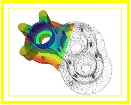
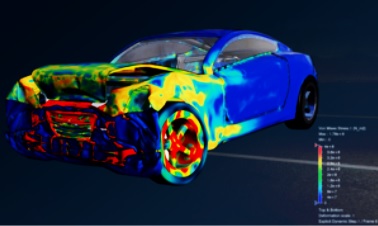
- Using FEM applications, one can simulate prediction accuracy in the chosen areas of the object much higher compared with the rest of the body structure. For example, in the car frontal-crash simulation, engineers can decide to increase the prediction accuracy of the front of the car compared to its back to save both computational time and cost. The figure shown below illustrates the car deformation in an asymmetrical crash in the simulation using finite element analysis by Dassault Systèmes.
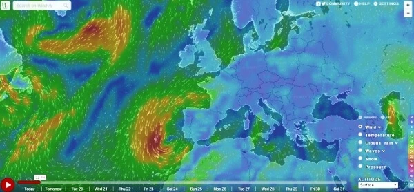
- Another example would be the weather forecast: it is possible and advisable to simulate areas above land rather than seas to have better prediction results with reduced computational energies unless needed otherwise. The figure below shows the screenshot of a simulation run by CFD to give a weather forecast.
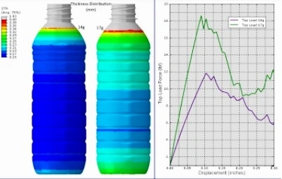
- Another FEM application lies in weight reduction, for instance, of a water bottle at Plastic Technologies Inc. (PTI). Using Abacus for running simulations, the company tested whether the bottle would buckle under top-loading conditions when it is light-weighted. Surprisingly, it was discovered that with the decrease in weight from 17g to 14 g, the top-load strength of the bottle decreased from 19 lbf to 12 lbf — a design consideration that embarked the company’s typical capitalist approach. The manufacturing company thereupon decided to modify the bottle’s design without significant delay.
One can assert, yet with great citational backing, that the most common users of the finite element method are the mechanical, automotive, and aerospace engineers. Other than structural problems, FEM covers problems immensely encountered in heat transfer, fluid mechanics, electromagnetism, biomechanics, geomechanics, and acoustics, among many others.
Its revolutionistic role in stiffness and strength visualization is worthy of admiration: it renders visualization possible in structurally crucial areas, such as where there are bends and twists.
FEM software which we enlisted in our CAD software article, offers tremendous simulation options for controlling the complexity of the problems and subsequently helping analysis via graphical representation, animation, contour plotting, parametric studies, vector field representation, report generation, and in other post-processing guises.
Furthermore, it helps tremendously not only by minimizing materials and weight but also prototyping costs. FEM does not deal with problems confined to their disciplines alone. That is, it also covers problems with multi-disciplinary considerations in which two or three fields of knowledge are strongly integrated. Its most typical example is the examination of thermal structure with the natural coupling of heat transfer and displacement. Another example includes aeroelasticity with the robust coupling between the external airflow and the distortion of the wing.
Applications of Finite Element Method (FEM) with Respect to the Engineering Problems
The finite element method classifies engineering problems into three distinct categories according to the characteristic features of such problems. These problems include:
- Equilibrium problems or time-independent problems
- Eigenvalue problems
- Time-dependent or propagation problems.
Let’s discuss each individually.
Equilibrium problems or time-independent problems
Most of the FEM applications fall in this category. In the equilibrium problems that come within the environs of solid mechanics, engineers need to determine the displacement distribution and stress distribution for a given mechanical or thermal loading.
Whereas, for equilibrium problems belonging to fluid mechanics, engineers are more interested in finding solutions in terms of pressure, velocity, temperature, and density distributions under steady-state conditions.
Eigenvalue Problems and Lastly
This category belongs to the Eigenvalue problems of solid and fluid mechanics. The problems encountered are the steady-state problems. For their solution, natural frequencies and modes of vibration of solids and fluids are determined.
The most typical examples of Eigenvalue problems that involve both solid and fluid mechanics are found in civil engineering, for instance, in problems concerning the interaction of lakes and dams. Apart from this, other examples appear in aerospace engineering, say, in problems associated with the sloshing of liquid fluids in solid tanks.
Lastly, this group of problems deals with the stability of solid structures and laminar flows.
Time-dependent or Propagation Problems
This category deals with problems that are commonly labeled as time-dependent or propagation problems of continuum mechanics.
It consists of problems that accompany the time dimension to the problems of the first two categories explained earlier.
Merits of the FEM
Some of the merits associated with FEM applications are better illustrated in the figure below.

Other benefits include efficient and less costly design cycles, equipment certification and verification, adaptability with a wide range of materials, lower R&D costs, and beyond.
Concluding Remarks
It can be distinctly asserted that every field of engineering is a potential user of FEM. But, because of the diversity of the nature of the pragmatics of problems, if it proves to be a useful technique for a particular problem in a particular discipline, it does not suffice to proclaim that it provides optimal solutions to all kinds of engineering problems. Therefore, over some time, several numerical and non-numerical techniques other than FEM have been developed to provide a more accurate approximate solution to the more complexified engineering problems.
Frequently Asked Questions
What is FEM and its applications?
It is a numerical technique that is used to solve partial differential equations and integral equations that define the current engineering problems. Physical principles and laws govern each problem, for example, the Euler-Bernoulli beam equation, Navier Stokes equations, and others. FEM is the technique of numerical integration of the PDEs and IEs to find an approximate solution.
What are the numerical integration techniques used most commonly in FEA?
Most of the time, the numerical integration in FEA is performed using standard techniques such as Runge-Kutta methods, Euler’s method as well as Adams-Bashforth, Adams-Moulton methods, and others.
What are the key areas of application of FEM?
Extensive applications of FEM are found in structural mechanics, heat transfer, fluid mechanics, fluid dynamics, electromagnetism, biomechanics, geomechanics, and acoustics, among many others.
What are the most common engineering problems encountered in FEM?
The three types of engineering problems encountered in FEM include equilibrium problems or time-independent problems, Eigenvalue problems, and lastly, time-dependent or propagation problems.
What are some merits of using FEM?
Some of the merits are virtual prototyping, low computational cost and time, graphical visualization, adaptability with a range of materials, dynamic loading, incorporation of boundary conditions, parametric modeling as well as certification and verification, higher productivity, increased revenue, and so forth.
I am the author of Mechanical Mentor. Graduated in mechanical engineering from University of Engineering and Technology (UET), I currently hold a senior position in one of the largest manufacturers of home appliances in the country: Pak Elektron Limited (PEL).