Basic Steps in Finite Element Method

The finite element method is a numerical technique that is used to approximate the solutions of complex engineering problems, which include, for instance, structural deformations (denoted by u in most cases) caused by applied loads. In problems such as these, exact solutions are somewhat impossible to determine. That’s why numerical methods such as FEM are most extensively employed in the design and optimization phase.

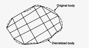
Finite element methods are based on the division of the body into smaller parts or regions, each being called the finite element. The concept according to which the engineering object is divided into finite regions is called discretization.

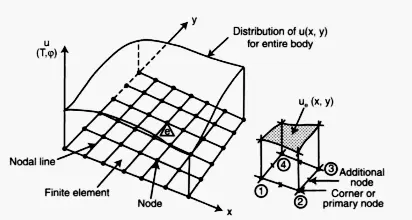
The benefit of such a division is that the distribution of the displacement is now also discretized into the corresponding sub-zones of the finite elements. That is, with the discretization of the body into finite zones, the displacement shall be assumed to be subsequently discretized into the respective sub-zones as well.

Another benefit is that these smaller regions or finite elements are now easy to examine and analyze in comparison to the entire body in terms of the distribution of u over it. The formulation and application of the finite element method (FEM) generally consists of eight essential steps. The present article is one effort, among others, to articulate these steps in a clear yet concise manner.

Steps in the Finite Element Method

Each step with its relevant discussion is presented below.

Discretization and selection of the element configuration

The first step in the finite element method is to discretize the body into smaller bodies called the finite elements. There are certain terms associated with these elements, as described below:

• Nodes or Nodal Points: The intersection of the sides of the finite elements is called nodes or nodal points. They are the vertices of the finite elements.
• Nodal line: The interface between the two nodal points along an axis is called a nodal line.
• Nodal plane: The interface between the two nodal points along an x-y plane is called a nodal plane.

It is worth noting that additional nodes can be introduced along the nodal lines or planes according to need.

But, some important questions should be raised: what should be the minimum size of each element? as well as, what type of elements should generally be used? and so on. These questions have everything to do with the characteristics of the continuum and the chosen idealizations or assumptions.

For example, if the body is idealized as a one-dimensional line, then the element we choose would be a line segment.

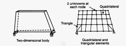
In the case of a two-dimensional body idealization, the element geometry would be of triangular or quadrilateral shape.

Likewise, for a three-dimensional body, the configuration would be a hexahedron with characteristic idealizations.

Furthermore, the body can be subdivided into regular-shaped elements in the interior. However, exceptions can be made if the boundary is of irregular shape. For complex boundaries, mathematical functions of higher degree are used to approximate them. In this vein, the concept of isoparametric elements is of central importance.

Selection of the approximation models or functions

The second step is to select the pattern or shape for the distribution of the unknown quantity that can be displacement or stress in stress-deformation problems, the temperature in heat-flow problems, fluid pressure or velocity, or both in fluid-flow problems, and so on.

The key point to understand at this step is that the nodal points of the element offer strategic points for writing mathematical functions. These functions (called the interpolation functions in most cases) are necessary descriptions related to the shape of the distribution of the unknown (u) over the entire domain of the element.

Most elementary forms of these mathematical functions are polynomials or the trigonometric series, polynomials being the simplest of the two due to the ease and simplification of their use in FEM.

If we denote the unknown (say displacement) by u, the respective interpolation function is thus written as follows:

u\;=\;u_1\;N_1\;+\;u_2\;N_2\;+\;u_3\;N_3+...+u_{m\;}\;N_m

Here, u₁, u₂, u₃ … u_m denote the unknown displacements at the nodal points 1, 2, 3 … m, and  N₁, N₂, N₃ … N_m represent the interpolation functions at the respective nodes.

For example, for a line segment with two nodes only, the unknowns or the degrees of freedom would be u₁ and u₂.

In the case of a triangular shape with three nodes, the unknowns would be u₁, u₂, u₃ … u₆ because two unknowns are associated with each nodal point.

The goal to be achieved at the end of the finite element method is to find out the unknowns u₁, u₂, u₃ … u_m at the nodal points 1 2 3 … m.

To meet that end, we therefore assume a shape or pattern in advance which it is hoped shall satisfy the conditions, laws, and principles of the existing problem.

The reader is encouraged to understand fully that the final solution would be in terms of the unknowns at the nodal points as the necessary consequence of the discretization process.

The figure shown below reveals that the final solution is necessarily a combination of the individual solutions in each element patched together at the shared boundaries. It is best illustrated through the cross-sectional view A-A (Figures A, B, C).

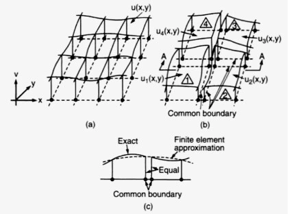
It signifies that the computed solution is not the same as the exact solution as marked by the solid line. Rather, it is always an approximate one shown by the dotted lines. Efforts are made to maintain a minimum gap between the two: the error is kept as low as possible.

Defining Strain-Displacement or stress-strain relationships

The third step involves defining certain quantities that are used in the principle intended for driving equations for the elements. One such principle is the principle of the minimum potential energy.

• In the case of stress deformation problems, one such quantity is strain. For a unidirectional body, the small strain along the y-axis is defined by the following expression:

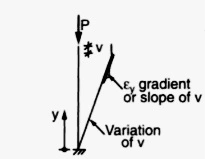
\in_y=\frac{dv}{dy}

Where v is the deformation in the y-direction.

In addition to strain, another significant quantity used subsequently is stress. It is defined by stress-strain law called the Hooke’s law as follows:

\sigma_y=E_y\;\in_y

Where σ_y is the stress along the y direction, and E_y is the elastic Young’s Modulus. The expression of stress is also defined in terms of displacements by substituting for E_y as follows:

\sigma_y=E_y\frac{dv}{dy}

• In the case of the fluid flow along the x-axis, the respective quantity is the gradient, which is defined as follows:

g_x=\frac{d\Phi}{dx}

Where is the fluid head, and g_x is the rate of change along the x-axis.

Likewise, the fluid velocity v_x for the fluid flow through porous media  is defined by Darcy’s law thus:

v_x=-k_x\;g_x

Where k_x is the coefficient of permeability and g_x is the gradient.

Deriving Element Equation

The fourth step being the most crucial, involves the use of laws and principles for deriving mathematical equations for the finite elements. These expressions come in general terms and are subsequently applicable to all the elements of the discretized body.

The two most common methods or alternatives used for deriving element equations are energy methods and weighted residual methods.

Energy Methods

The energy methods are based on the concept of the consistent states of the loaded body, that is the stationary values of the scalar quantity, such as energy or work. The derivation of the expressions governing these stationary states of energy requires the intensive use of the variational calculus, whose brief description shall be presented here.

Before proceeding further, it is key to mention some crucial energy methods and variational principles. These include the principle of stationary potential and complementary energies, Reissner’s mixed principle, and hybrid formulations, among many others.

The stationary value of a function F(x) assumes the maximum, minimum, or saddle point of a function. Under certain unique or characteristic conditions, the function implies only the maximum and minimum values. In that case, the derivative of the function F is equal to zero.

\frac{d(F)}{dx}=0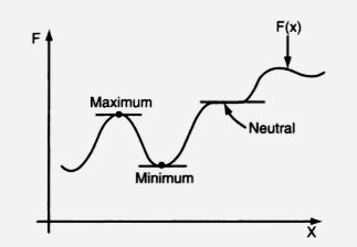

But what is this function F(x)? It is the potential energy function, or more simply, the potential energy of the loaded body is represented by the function F.

In the present case, for example, assume a body in the form of a column under loaded conditions, as shown in the figure. If it is static and under equilibrium conditions, one can easily state that its potential energy is minimum. Potential energy here is denoted by p and defined as follows:

{\mathrm\pi}_p=\mathrm U\;+\;{\mathrm W}_{\mathrm p}

The above mathematical expression explicitly states that the potential energy of the mentioned column is the algebraic sum of the internal strain energy (U) and the potential of the external loads W_p, which is defined as the capacity of the external loads (P) applied on the column to cause deformation (v) in it by performing some work.

According to the principle of the minimum potential energy, if the column has the stationary value of potential energy, its derivative must be equal to zero.

\frac{\delta{\mathrm\pi}_p}{\delta x}=0

Or,

\delta U-\delta W=0

Here, δ shows the variation of the potential energy or a series of partial derivatives.

The relation between the potential of the external loads and the work done is given by the following expression.

\delta W=-\delta W_p

The negative sign here in the last two equations implies that the potential of the external loads is lost in the form of the work done by the external loads.

For the verification of the minimum value of potential energy, its second derivative must be greater than zero, proof of which is beyond the scope of the current text.

\delta^2\;{\mathrm\pi}_p\;=\;\mathrm\delta^2\;\mathrm U\;-\;\mathrm\delta^2\;{\mathrm W}_{\mathrm p}\;>\;0

Here, δ stands for the variation or a series of partial differentials. More simply, it denotes the derivatives of p for the unknowns (u).

As π_p the function of the unknowns (u), for example, one can write;

{\mathrm\pi}_p\;=\;\mathrm\pi({\mathrm u}_1,\;{\mathrm u}_2,\;{\mathrm u}_3,......,{\mathrm u}_{\mathrm n})

Now, According to the principle of the minimum potential energy as elaborated above implies π_p=0,

Or,

\frac{\delta\pi_p}{\delta u_1}=0

\frac{\delta\pi_p}{\delta u_2}=0

\frac{\delta\pi_p}{\delta u_3}=0

.

.

.

\frac{\delta\pi_p}{\delta u_n}=0

From these equations, one can calculate the unknowns u₁, u₂ … u_n.

Method of Weighted Residuals

Another method used for deriving element equations is the method of weighted residuals (MWR). It employs various schemes such as collocation, subdomain, least squares, and Glarkin’s method. Among the four, Glarkin’s method gives results identical to those obtained from the variational procedures and is only one of the most commonly used MWR methods in FEM applications.

This principle is based on the minimization of the residual (defined as the error between the actual and approximate solution) once the approximate solution is put into the differential equations that govern a problem.

Example of MWR

For example, consider the following differential equation that governs the problem:

\frac{\delta^2\;u^\ast}{\delta\;x^2}\;-\;\frac{\delta\;u^\ast}{\delta t}\;=\;f\left(x\right)\;...\;(1)

Here,

u* = Unknown

x = coordinate

t = time

f = forcing function

In short form, the above equation is written as:

L\;u^\ast\;=\;f\;...\;(2)

where,

L\;=\;\frac{\delta^2}{\delta\;x^2}\;-\;\frac\delta{\delta t}

and is called the differential operator.

Let’s denote the approximate solution of u* by u and define it as follows:

u\;=\;\varphi_0\;+\;\sum_{i\;=\;1}^n\;\alpha_i\;\varphi_{i\;}...\;(3)

u\;=\;\varphi_0\;+\;\alpha_1\;\varphi_1\;+\;\alpha_2\;\varphi_2\;+...+\alpha_n\;\varphi_n

Here,

\varphi_1,\;\varphi_2,......,\varphi_n

are the known functions and are selected keeping in view the existing boundary conditions. Where, 0is a unique function that satisfies the essential geometric/forced boundary condition (detail below in the next steps). The coefficients α₁, α₂, …, α_n are yet to be determined subsequently.

Again, in short form, the above equation is rewritten as follows:

v\;=\;\sum_{i\;=\;1}^n\;\alpha_i\;\varphi_i\;...\;(4)

Where,

\alpha_1\;=\;1

and

\varphi_1\;=\;\varphi_o

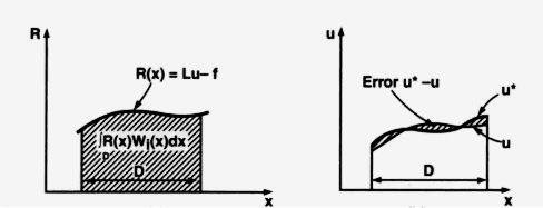
We get the residual R(x) after the approximate solution u is put into equation (2).

R(x)\;=\;Lu\;-\;f\;...\;(5)

The residue is zero if u=u*, which is not the practical case.

In the MWR method, as stated above, the aim is to keep the value of the R(x) as minimum as possible to reduce error. For that purpose, various schemes are used, such as least squares, Glarkin’s method, and others.

For the sake of simplicity, we do not delve into one particular method here but reproduce one general equation of these methods below.

\int_DR(x)\;W_i(x)\;d(x)\;=\;0\;...\;(6)\;\;\;\;\;\;\;\;\;\;\;\;\;i\;=\;1,2,3,\;...\;,n

The above-written equation gives the idea about the minimization of R(x).

Here, D denotes the whole domain of the body under analysis, and Widenotes the weighting functions. Different MWR schemes define weighting functions differently.

For example, in the collocation method, W_i=1, which implies that the weighted value of the residue R(x) vanishes over the whole domain D of the body.

The graphical representation of equation 6 is shown below. The shaded area shows the error caused by the difference between u* and u.

Let’s consider an example governing a one-dimensional stress-deformation problem in a column of length L. The following partial differential equation defines the problems in the column.

c\frac{d^2\;v^\ast}{dy^2}\;=\;f\;...\;(7)

Here,

v* = Unknown

y = coordinate

c = material property

f = forcing function

c\frac{d^2\;v^\ast}{dy^2}\;=\;10\;...\;(8)

If v denotes the approximate solution for v*, then equation 3 can be re-written as a special case as follows:

v\;=\;a_1\;+\;a_2\;y\;+\;a_3\;y^2\;=\underset{}{\sum\alpha_i\;\varphi_{i\;}\;...\;(9)}

Here,

\varphi_1\;=\;1,\;\varphi_2\;=\;y\;and\;\varphi_3\;=\;y^2

Equation 9 is not selected in the air. Rather, it must satisfy the boundary conditions of the problem at hand.

Let’s now calculate the residue. For that purpose, substitute approximate solution v for the exact solution v* in equation 8 and take their difference.

R(y)\;=\;\frac{d^2v}{dy^2}\;-\;10\;...\;(10)

According to the method of the weighted residuals (MWR), as we learned above, the following statement defines the idea about the minimization of the residue.

\int_0^LR(y)\;W_i\;(y)\;dy\;=\;0\;\;\;...\;(11)\;\;\;\;\;\;\;\;where\;i\;=1,2,3

Or,

\int_0^L(\frac{d^2v}{dy^2}\;-\;10)\;W_i\;(y)\;dy\;=\;0

Or,

\int_0^L\left(\frac{d^2\;{\displaystyle\sum_{}^{}}\;\alpha_i\;\varphi_i}{dy^2}\;-\;10\right)\;W_i\;(y)\;dy\;=\;0\;...\;(12)

Now, differentiate equation 9 twice and substitute it in equation 12, yielding the following three simultaneous equations.

\int_0^L\left(\frac{d^2\;{\displaystyle\sum_{}^{}}\;\alpha_i\;\varphi_i}{dy^2}\;-\;10\right)\;W_1\;(y)\;dy\;=\;0

\int_0^L\left(\frac{d^2\;{\displaystyle\sum_{}^{}}\;\alpha_i\;\varphi_i}{dy^2}\;-\;10\right)\;W_2\;(y)\;dy\;=\;0

\int_0^L\left(\frac{d^2\;{\displaystyle\sum_{}^{}}\;\alpha_i\;\varphi_i}{dy^2}\;-\;10\right)\;W_3\;(y)\;dy\;=\;0

When the above three simultaneous equations are solved, the values α₁, α₂, …, α_n are obtained. Putting these values back into equation 9 gives the approximate solution v for v*.

Finally, the use of the energy methods and the weighted residual methods give equations that describe the behavior of the elements, which can be thus expressed in the concise form as follows.

\left[k\right]\{q\}\;=\;\left[Q\right]\;...\;(13)

Where,

[k] = element property matrix

{q} = vector of unknown at the nodes

[Q] = vector of element nodal forcing parameters

For stress-deformation problems, one can re-define thus:

[k] = stiffness matrix

{q} = vector of nodal displacements

[Q] = vector of nodal forces

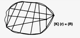
Assembling element equations to get global equations and introducing boundary conditions

In this crucial step, the equations governing the entire body are defined. These equations approximate the behavior of the entire body in question. The use of the variational and the residual method are important in this regard as discussed and applied in the previous step. 

Once the equations defining the behavior of an element are established, it is easy to recursively use this equation over and over again for all the elements of the discretized body, thus adding them finally to get global equations according to the law of compatibility or continuity according to which the neighboring elements must remain in the neighborhood of each other after the load is applied. That is, the displacements of the two adjacent points must be of the same value (Figure below).

Hence, the global assemblage equations obtained are expressed in the matrix form as follows,

\left[K\right]\{r\}\;=\;\left[R\right]\;...\;(14)

Where,

[k] = assemblage property matrix

{q} = assemblage vector of nodal unknowns

[Q] = assemblage vector of nodal forcing parameters

Applying Boundary Conditions

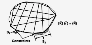
Equation 14 gives an explanation for the capability of a body to withstand applied loads. But under what constraints? This crucial step involves the incorporation of such constraints, commonly known as boundary conditions.

In engineering problems, the boundary conditions include both the surroundings and the structural (or thermal or electrical) constraints, without which it is impossible to analyze the behavior of a body or structure correctly. The figure below shows the body without boundary conditions.

More simply, they are physical constraints or supports to help the structure stand in space. As shown in the figure below, on the boundaries S₁ and S₂, two boundary conditions are defined in terms of the known values of the unknowns.

As shown below, the supported beam, which is centrally loaded, defines the boundary by joining two endpoints where displacements are restrained. Such boundary conditions, which are articulated in terms of displacements, are known as essential, geometric, or force boundary conditions.

A supported beam that is provided with simple supports has zero bending moment at the two extreme ends. That is, the second derivative of the displacement is zero at the supporting ends. Such boundary conditions are known as natural boundary conditions.

When we incorporate the boundary conditions into equation 14, then it has to be modified a bit only if such boundary conditions are the geometric boundary conditions. The incurring change is here represented by putting overbars as shown in equation 15.

\left[\overset-K\right]\{\overset-r\}\;=\;\{\overset-R\}\;...\;(15)

Solving for the primary unknowns (displacements)

Equation 15 constitutes a set of linear or nonlinear sets of simultaneous equations which, when expanded, take the following standard form.

k_{11}\;r_1\;+\;k_{12}\;r_2\;+\;k_{13}\;r_3\;.......\;k_{1n}\;r_n\;=R_1

k_{21}\;r_1\;+\;k_{22}\;r_2\;+\;k_{23}\;r_3\;.......\;k_{2n}\;r_n\;=R_2

.

.

.

k_{n1}\;r_1\;+\;k_{n2}\;r_2\;+\;k_{n3}\;r_3\;.......\;k_{nn}\;r_n\;=R_n

These algebraic simultaneous equations can be solved by using the Gaussian elimination method or the iterative method for the primary unknowns (displacements) r₁, r₂, …, r_n. In stress-strain problems, the primary unknowns would be stresses, whereas in the case of fluid flow problems, they would be fluid head or velocity head.

Solving for secondary quantities

At this stage, using the primary quantities, the secondary quantities would be calculated.

In the case of stress-deformation problems, the secondary quantities can be strains, stresses, bending moments, shear forces, and others. They can be determined using the primary quantities with the help of equations defined in step 3.

Interpreting the results

This is the last step. Its main purpose is to reduce the results of the finite element method into a form that can be used for engineering analysis and design.

The results obtained at the end of FEM are usually received in the form of a printed output. Following this, the critical sections of the body or structure are marked, and the values of displacement and stresses are plotted or tabulated for a rational engineering analysis.

Frequently Asked Questions

Zain ul Abedin

I am the author of Mechanical Mentor. Graduated in mechanical engineering from University of Engineering and Technology (UET), I currently hold a senior position in one of the largest manufacturers of home appliances in the country: Pak Elektron Limited (PEL).