The exponential rise in the cost of fluid flow analysis, for example, in aircraft development, has been undoubtedly a serious concern. One of the major factors contributing to this rise in cost is attributed to the evaluations of the multiple design modifications to reach a final design that is reliable enough in terms of meeting all the required performance characteristics.
The design evaluations made through wind tunnel experiments are not only costlier but also much more time-consuming. In this vein, modern means such as computational simulations in the form of computational fluid dynamics (CFD) have emerged to be recognized worldwide as an authentic horizon for testing engineering objects with reduced costs and time.
What is CFD?
Computational fluid dynamics (CFD) is one among many computational approaches that analyze fluid flow by solving complex fluid equations on a digital computer. Its codes are diverse and applicable for investigation in numerous fields for fluid motion (momentum) and energy analysis.
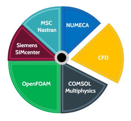
CAD Softwares used for CFD computations include ANSYS Fluent, COMSOL Multiphysics, OpenFOAM, CFD++, Simcenter STAR-CCM+, NUMECA FINE/Open, Autodesk CFD, SolidWorks, and others.
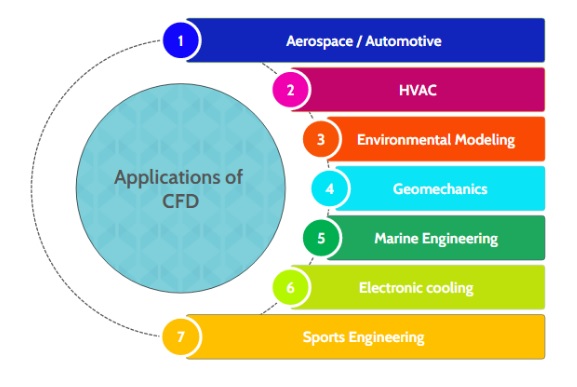
The encompassing fields that come under the scope of CFD analyses include turbomachinery, aerospace science, geomechanics, biomechanics, sports engineering, automotive engineering, and others, as outlined below.
Merits of CFD
It would not be wrong to say that with the emergence of CFD programs as a robust tech tool for investigating fluid phenomena, experts are now at much ease due to getting free from the constraints of time and expensive resources. Other benefits include high predictive capability and graphical visualization of results, among many others, as shown below.

Numerous CFD codes are available today for use in the development of, for instance, aircraft of any configuration. The sophistication of these codes is due to the complexity of the mathematical model employed and, thereby, in their encoded ability to examine the underlying fluid phenomena.
These codes are based on complex fluid dynamic equations. One among many of these equations is a set of Reynold-Averaged Navier-Stokes equations (RANS) on which many of the CFD codes are based. On top of these, Navier-Stokes equations are even more extensively used, which we shall discuss a little later.
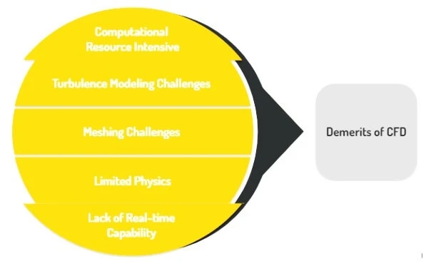
Demerits of CFD
The CFD codes are very effective in simulations proper to fluid flow. Today, most of the credible research papers published in well-reputed journals are structured on CFD modeling. They demonstrate exceptionally impressive computations on complex geometries. Yet, there are also certain limitations associated with CFD simulations, and they include the following:
- Large computational time and storage
- Inadequacies of the turbulence modeling
Experts realize that no doubt CFD has made analyses much easier than ever before, yet it is also equipped with certain quantifiable limitations such as enormous space for file storage, large times required for computations, and unreliable simulation results often associated with the inadequacies of turbulence modeling. Some of the demerits of CFD are illustrated below.
Challenges in CFD Modeling
By these inadequacies, one means inherent difficulties in modeling complex phenomena of turbulent flow due to a number of factors, such as:
- Reynolds-averaging assumptions
- Modeling wall-bounded flow
- Model sensitivity to flow conditions
- Unsatisfactory treatment of the unsteady turbulence
- Sensitivity to mesh quality, etc.
What are Navier-Stokes (N-S) Equations?
Scholars are well familiar with the fact that today, the widely used CFD methods include inviscid approximations to the Navier-Stokes equations. What? What are these equations?
They are the expression of Newton’s second law of motion and a constitutive law that links fluid stresses with the volume and shape distortions that the material elements of the fluid undergo in a Newtonian fluid.
They are written for both compressible and incompressible fluids. In hydraulics and related engineering applications, mostly N-S equations for incompressible fluid flow are encountered. However, with the introduction of gas to these equations, the resulting expressions won’t be much different.
For simplicity, we articulate below four expressions of Navier-Stokes equations for a viscous fluid motion.
Momentum Equations
x-direction
\rho\left(\frac{\delta u}{\delta t}\;+\;\mu\frac{\delta u}{\delta x}\;+\;v\frac{\delta u}{\delta y}\;+\;w\frac{\delta u}{\delta z}\right)=-\frac{\delta p}{\delta x}+\;\rho g_x\;+\;\mu\left(\frac{\delta^2\mu}{\delta x^2}\;+\;\frac{\delta^2\mu}{\delta y^2}\;+\;\frac{\delta^2\mu}{\delta z^2}\right)y-direction
\rho\left(\frac{\delta v}{\delta t}\;+\;\mu\frac{\delta v}{\delta x}\;+\;v\frac{\delta v}{\delta y}\;+\;w\frac{\delta v}{\delta z}\right)=-\frac{\delta p}{\delta y}+\;\rho g_y\;+\;\mu\left(\frac{\delta^2v}{\delta x^2}\;+\;\frac{\delta^2v}{\delta y^2}\;+\;\frac{\delta^2v}{\delta z^2}\right)z-direction
\rho\left(\frac{\delta w}{\delta t}\;+\;\mu\frac{\delta w}{\delta x}\;+\;v\frac{\delta w}{\delta y}\;+\;w\frac{\delta w}{\delta z}\right)=-\frac{\delta p}{\delta z}+\;\rho g_z\;+\;\mu\left(\frac{\delta^2w}{\delta x^2}\;+\;\frac{\delta^2w}{\delta y^2}\;+\;\frac{\delta^2w}{\delta z^2}\right)The continuity equation (Conservation of mass)
\frac{\delta u}{\delta x}\;+\;\frac{\delta v}{\delta y}\;+\;\frac{\delta w}{\delta z}\;=\;0Here,
- u, v and w are the x, y and z components of velocity
- p is fluid pressure
- ρ is density
- μ is the dynamic viscosity
- gx, gy and gz are the external force components along x, y, and z axis
- t, x, y, and z are the time and spatial coordinates
The above three mathematical expressions are called the Navier-Stokes Equations frequently used in CFD modeling. They were named after the French Mathematician L.M.H Navier (1758-1836) and English mechanician G.G. Stokes (1819-1903).
These three equations, when combined with the fourth continuity equation or the conservation of mass equation
\frac{\delta u}{\delta x}\;+\;\frac{\delta v}{\delta y}\;+\;\frac{\delta w}{\delta z}\;=\;0give a complete description of the flow of the incompressible Newtonian fluid.
Precisely, one can state that:
The first three questions state the conservation of momentum in fluid flow along each coordinate, thus defining pressure forces, viscous forces, and external forces. Whereas the fourth equation states the conservation of energy. It describes that the sum of the partial derivatives of the three components of velocity with respect to their spatial coordinate is zero.
Hence, one can fairly read that there are four unknowns here in the N-S equations: u, v, w, and p. Due to the general complexity of these nonlinear second-order differential equations, exact solutions are impossible to achieve except in certain unique instances in which the solutions obtained are in close agreement with the experimental results. Summarizing this, the Navier-Stokes equations are the governing differential equations of motion proper to the incompressible Newtonian fluids.
Essential Steps of CFD Simulations/Modeling
The CFD codes solve the Navier-Stokes equations using numerical methods because the analytical methods fail to tackle such complex problems. Similar to FEA/FEM used in the analyses of the structural problems and involve a systematic procedure, CFD modeling of the fluid flow follows few essential steps in providing numerical solutions to the N-S equations. These include:
- CFD codes break the mentioned Navier-Stokes continuous equations into discrete equations and break the spatial and temporal domains into a grid/mesh.
- Now, the partial derivatives are replaced with close approximations.
- After that, boundary conditions that define the fluid behavior at the boundaries are applied.
- Solvers then solve the discrete equations using iterative methods numerically until a converged solution is obtained.
- Finally, in the post-processing phase, all the useful information is extracted, like velocity profile, pressure distribution, and so forth, to ease visualization for subsequent analysis and drawing intended results.
Frequently Asked Questions
What is CFD?
It stands for Computational Fluid Dynamics. It is a branch of fluid mechanics. It provides computer-based approximate solutions to the complex engineering problems that concern fluid flow in terms of, for instance, momentum and energy.
What are the merits and demerits of using CFD simulations?
Merits of using CFD simulations include reduced computational time and space, optimized design, reliable results, predictive modeling, flow pattern visualization, and others. Whereas demerits are inadequacies of turbulence modeling, meshing problems, limited physics, and so forth.
What are the Navier-Stokes Equations?
They are the expression of Newton’s second law of motion (three momentum conservation equations) and a constitutive law (one mass conservation equation) that links the fluid stresses with the volume and shape distortions that the material elements of the fluid undergo in a Newtonian fluid.
I am the author of Mechanical Mentor. Graduated in mechanical engineering from University of Engineering and Technology (UET), I currently hold a senior position in one of the largest manufacturers of home appliances in the country: Pak Elektron Limited (PEL).