Geometric Modeling and its Various Types

CAD/CAM systems were principally designed to offer the graphical representation of the object under design and manufacturing, for which these systems initially relied heavily on the drafters until recently.

Due to the rapid development in the field of computer graphics and since geometric models developed by the drafters did not give an unambiguous representation of their corresponding objects, they were soon relinquished for complex engineering analyses and applications.

Now, the pressing need is to foster a CAD/CAM/CAE climate in which the resulting geometric models would be unique and all-encompassing to virtually all engineering functions, ranging from documentation to engineering analysis to manufacturing.

What is geometric modeling?

It refers to the methods used in the creation of the exact geometric model of an engineering object in the computer system.

Why geometric modeling?

Geometric modeling is the heart and soul of any CAD/CAM/CAE environment. Its importance in the CAD/CAM realm is the same as those of governing equilibrium equations in the classical engineering fields such as mechanics and fluidics.

But, today, it is an open engineering secret that the modeling of an object alone, if not fully, then partly, is of little or no importance unless it generates enough database for its subsequent utilization by the engineering applications module.

Requirements of Geometric Modeling?

The product design originally appears in the designer’s mind, who translates this design on paper by making product drawings for the manufacturing engineer to plan the necessary operations required in the manufacturing process.

In the earlier days, product/part drawings were made along with the prototypes to disseminate the needful information. But, today, in a densely complicated computerized landscape,  the information a designer or a drafter generates must be readily accessible to some other elements of a CAM system.

Thus, a geometric model should be as clear and comprehensive as possible for its optimal utilization by the other modules of the modeling and manufacturing system.

Moreover, such a geometric model should be equipped with functions such as design, analysis, drafting, manufacturing, production engineering, inspection, testing, and quality control.

Types of Geometric Molding

There are different types of geometric models of an object in the CAD/CAM systems. Traditionally, there are three types of geometric models, namely wireframe model, surface model, and solid model, as shown in the figure below for the same object and described next.

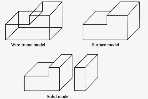
Wireframe model

The geometric model that uses the network of interconnected lines or wires to express the edges of a physical object being modeled is known as a wire frame model. It is also called an edge-vortex or stick figure model.

It represents the simplest form of a geometric model as it requires relatively less time and memory to create the computer models of parts, particularly in computer-assisted drafting systems. It would be thus used to automatically generate the cutter paths necessary to drive the NC machine tool for part manufacturing.

There are certain demerits linked to the wireframe model. Although it provides necessary information about the location of the surface discontinuities on the part, it does not give a complete description quite often.

Secondly, the wireframe models provide little information, if any, specific to the part surface: They do not distinguish the part’s exterior from its interior.

The figure shown below elaborates on the procedure needed to generate the wireframe model of a rectangular object. Like most of the CAD/CAD systems, the current image, as illustrated below, gives a split screen approach to display three orthogonal and one isometric view of the object.

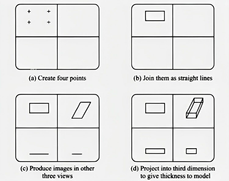
A step-by-step procedure is explained below:

1. In the first step, four points (+) are marked to indicate the top view to represent one of the faces of the modeled rectangular block.
2. In the second step, the points are joined by straight lines to show the edges of the top view of the rectangular object.
3. In the third step, the drawn image is now projected into three other views: one isometric and two orthogonal.
4. In the fourth final step, the face is projected into the third dimension as the thickness of the rectangular object.

Surface Model

Many of the ambiguities of the wireframe model are resolved in the surface model. A surface model is created by connecting various surface elements or by defining distinct surfaces to represent part geometry. 

These surface elements include descriptions in terms of points, edges, and faces between the edges. Some CAD/CAM systems are equipped to provide certain surface features to construct part geometry of which plane is the most simple form.

The surface modeling systems can calculate surface intersections and surface areas. Few such systems are able enough to produce shaded images and remove hidden lines automatically.

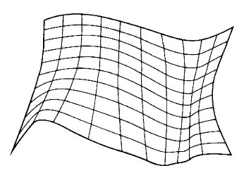
In many surface modeling practices, two different types of spline curves (best approximate curves) are used to generate surface patches. These two include Bezier curves and B-spline curves. Others include NURBS and T-splines.

Let’s discuss each in a little detail.

Bezier Surface

A Bezier surface is named after the French engineer Pierre Bezier, who used these parametric curves in the 1960s and developed them further later on to design automobile body surfaces.

There are some serious problems with the cubic (Hermite ) spline. This piecewise cubic function (three-degree polynomial) that interpolates a set of data points and guarantees curve smoothness at all data points is simple, yet it isn’t easy to control.

The Bezier curve is unique in a way that it passes only through the first and last data points (instead of passing through all data points as in cubic splines) while approximating all the interior ones.  

The construction of the Bezier curve in this way makes it easy to sculpt natural surfaces such as automobile body panels/surface patches.

In the figure shown below, a Bezier curve is manipulated by four control points, P₀, P₁, P₂, and P_3, also known as control vertices. As stated above, it interpolates only through the first and last data points (0 and 3) and would approximate (the rest of ) the interior points (1 and 2).

More precisely, when manipulated, the Bezier curve would pull to the interior points without passing through them. The tangent to the curve at P₀ would be given by P₁-P₀, while the tangent at P_n by P_n-P_n-1.

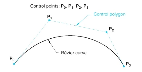
The control polygon is formed, as shown by connecting all the control points in a correct sequence. It is noteworthy how strikingly the control polygon suggests the shape of the Bezier curve.

It is also key to note that the degree of the Bezier curve is always one less than the number of the control points. In the present case, there are four control points or control vertices, implying that the degree of the curve would be 3; that is, it would be a cubic polynomial.

The table manifested below elaborates on the degree of different Bezier curves and their control points.

Bezier Curve	Degree	Control Point
Linear	1	2
Quadratic	2	3
Cubic	3	4
Quartic	4	5
Quintic	5	0

Lastly, there is one key concept known as a convex hull. The figure shown below illustrates the control vertices, control polygon, and convex hull of a Bezier curve.

The convex polygon formed by stretching a rubber band through all the control vertices of the control polygon is known as the convex hull. The Bezier curve lies fully within the convex hull. No two Bezier curves intersect if their convex hulls do not intersect. In case their convex hulls intersect, it is first seen whether the Bezier curves intersect or not.

But, there are also certain problems with the Bezier curves. 

1. As the number of control points forming the curve increases, the degree of the curve also increases. We know that curves with higher degrees are not that easy to control as they tend to oscillate.
2. There is no local control of the Bezier curve: Moving one control point would affect the entire curve.

B-splines

Two of the shortcomings of the Bezier curves, as stated above, namely, sheer reliance in the determination of the polynomial degree of the Bezier curve on the number of the control points as well as the absence of local control over the shape of the curve, are well addressed by B-splines.

They are non-global; that is, they provide needful local control over the geometry of the curve. Moreover, now, the degree of the curve is independent of the control points.

So, what is a B-spline? It is a composite of several curves such that different curve spans are connected at knots. The sole philosophy behind this splitist approach is to break down the monopoly of the control points over determining the polynomial degree of the curve. Now, each curve span of a B-spline curve would have k number of control points, and thereupon the degree would be k-1.

In the construction of a B-spline, the first curve span is generated using its k number of control points, then the second span using its different k points by dropping the previous ones, and so on until the last curve span is defined using its k points.

For better understanding, let’s discuss a B-spline with different construction definitions using five control points.

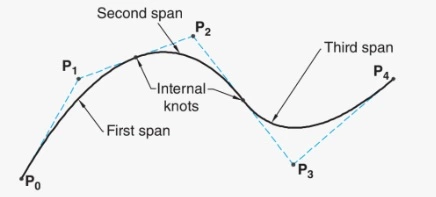
• In the figure shown below, the B-spline consists of three curve spans joined together by two internal knots. The curve has 5 control points with k=3 because the curve (-span) is quadratic-polynomial (of degree two).

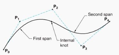
• The B-spline is now shown to have consisted of two curve spans joined together by a single internal knot. The curve has the same 5 control points with k=4 because the curve (span) is cubic polynomial (of degree three).

• Next, the B-spline is drawn using four curve spans (now straight lines) joined together by three internal knots. The curve has the same 5 control points with k=2 because the curve (span) is perfectly linear.

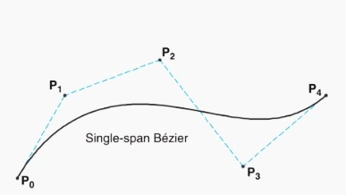
• Finally, the B-spline is constructed to be the same as a single curve span. The control points are 5 as above, with k also equal to 5 because the curve (span) is quartic-polynomial (of degree four).

From all the B-splines discussed before, one can fairly say that the degree of the curve is not the function of the control points: With 5 control points in each one of the four cases, the degree of the curve may be 2, 3, or 4.

Upon closely reading the afore-shared illustrations, there is one thing that seeks attention: In all four cases, the algebraic sum of the number of spans and the degree of the polynomial is equal to 5 (total control points). For that purpose, all the B-splines are reproduced on the same plot in the figure below.

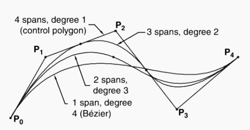
Here lies one result: if the degree of the curve is one less than the number of control points (as shown in the final figure), the B-spline is identical to the Bezier curve. In that case, there is a single curve span without any internal knot, and all the control points are used. Thus, one can ascertain that a Bezier curve is one special case of the B-spline. 

If the internal spacing between the neighboring knots is equal, or precisely, if the curve has uniform knot spacing, it is known as uniform-rational B-spline. All the cases discussed above have uniform knot spacing.

But in general case, the nonuniform-spacing offers a more pragmatic approach to editing a curve by adding or deleting internal knots. Curves such as this are known as nonuniform B-splines (NUBS) compared to NURBS, which will be elaborated next.

To summarize, one can write that a B-spline curve-span (also known as a surface patch) permits local control, as moving one point would not affect the resultant geometry of the B-spline (figure below).

Or precisely, the polynomial degree of the B-spline is now independent of the number of control points since the impact of changing a control point would be only localized. Furthermore, the degree of the curve (or the surface patch) can now be changed without altering the number of control points.

NURBS

As already discussed, the nonuniformly spaced internal knots structure the nonuniform B-splines (NUSB). They are not the same as nonuniform rational B-splines (NURBS). The word rational is yet to be incorporated into the concept of NUBS.

The nonuniform rational B-splines are defined by a rational formula consisting of homogeneous coordinates, which is a complex phenomenon and lies beyond the scope of the present article.

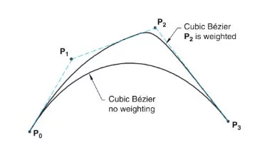
In a nutshell, in the NURBS, the control points are weighted to control the shape of the curve as desired. Strictly speaking, on increasing the weight of the control point, the curve tends to get pulled to that control point. In some cases, it may completely interpolate the control point as well. The figure below demonstrates how a weighted control point controls the shape of the cubic Bezier curve by dragging it toward it.

Capable of representing not only freeform shapes but also analytic forms (such as lines, curves, cones, etc.), the rational B-splines provide a single precise mathematical form to enable such graphic representation. They can represent both B-splines and Bezier curves.

In short, NURBS curves define surfaces that use rational B-splines. They include weighing value at each point on the curve, thereby rendering some points more influential and decisive over the shape of the final curve compared with other points. It helps thus creating a plethora of surfaces than possible with the regular B-spline.

But, there is not everything well with the NURBS surfaces. The reason is that all the NURBS surfaces have rectangular topology, as illustrated below. The control mesh defining a NURBS surface contains four edges and two parametric directions, u and v. Isoparametric curves, also known as isoforms on the surface, are defined by setting either u or v to a constant value.

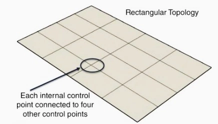
Every control point is simultaneously connected to four other control points in the NURBS surface. To add localized detail to the surface, therefore, requires the addition of more isoforms, which regrettably increase the number of control points needed to manipulate the surface, with many of them containing no significant geometric information but acting as a topological necessity to satisfy some topological constraints.

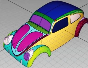
Secondly, due to the rectangular topology, various NURBS surfaces are joined to form a complex surface or watertight body. The figure below shows a car body made into several surface patches.

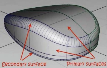
Another figure (below) shows a device housing that is made of joining primary surfaces (top, bottom, and side) with the mediation of the secondary surfaces (blend fillet).

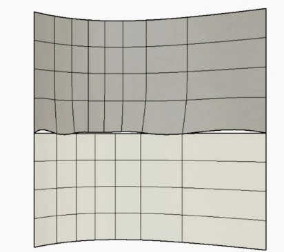
As a result of this surface quilting of the two mating surfaces, small gaps are left in between surface patches. They must be eliminated in the transition phase from design to analysis to manufacturing. But, doing so squanders a lot of precious time and requires expensive surface repair routines.

T-Spline

First defined by Thomas W. Sederberg in 2003, the use of T-spline was commercialized in 2004 with the founding of T spline, Inc. In 2007, a US patent related to T-splines was awarded. This technology was acquired by Autodesk in 2011 which incorporated it in Autodesk Fusion 360.

T-splines resolve the problems associated with the NURBS surfaces counted above, such as related to the formation of a uniform grid of UV curves throughout the surface, rectangular geometry thereby necessitating the designer to break the geometry into several individual small surface patches, and finally the development of gaps between the patches.

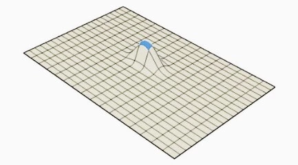
T-splines offer local refinement by introducing only a limited number of control points. They are capable of producing single, unified surfaces that are smooth and continuous and are easy to thicken or shell. They are free of inter-patches gaps.

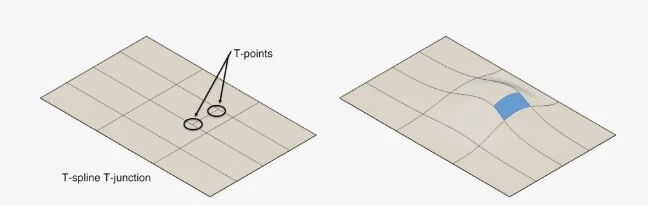
So, what is T-Spline? It is a nonuniform rational B-spline that allows T-junctions at T points. As shown in the figure below, the use of T-junctions implies that a row of control points can be eliminated without stretching or kinking the surface. Such a surface is called a T-spline because the partial rows of control points end in T-points.

More precisely, the use of T-splines supports the addition of necessary details or complexity to the curve surface without traversing it across. In the mathematical jargon, the T-points are called curvature continuous C².

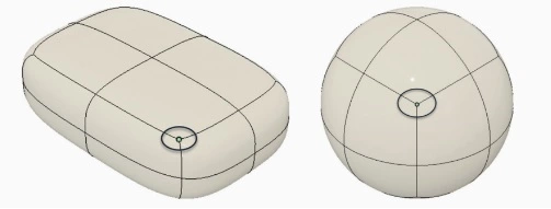
Moreover, T splines are also known to have star points as shown in the figure below for both box and quadball primitives. These are the control points when three, five, or more edges come together to form a junction. They are mostly generated by extruding the face. They are how T-splines change from a rectangular to an arbitrary topology in which there are no cumbersome efforts required for the creation of single individual surface patches to ensure surface smoothness and geometric continuity.

Furthermore, star points give more design freedom to the engineer for employing modeling techniques such as extrusion, surface deletion, and merging the surfaces among others.

But, there lies a problem: the shape of the T-spline is somewhat difficult to control at star points. Careful selection of star-points such as on flat surfaces can help avoid this design difficulty.

Solid Model

Over the past twenty years, the field of solid modeling as a means for representing objects as solids has been subject to ample research, and it continues to remain so since the intended objectives have not yet been achieved.

Solid modeling is the natural extension essentially drawn from the use of unidirectional entities (curves) or bi-directional entities (surfaces) to think in terms of modeling objects using three-dimensional solids.

The programs or software thus used are known as solid modelers or volume modelers and are built to hold unambiguous representations of the geometry of several solid objects.

Solid modeling leads the design engineer or the designer to a world of greater realism and enhanced possibilities. Since the object’s surfaces are mathematically represented, the mass between them is also defined…

A complete set of information inhered in the solid model is advantageous to the automatic production of realistic images of a shape as well as the automation of the process of interference checking.

Moreover, there can be written new application programs at a letter stage that help exploit the completeness of the solid model to lessen or eliminate the need for user intervention in design analysis (FEA) and manufacturing tasks (developing G-code programs for NC machining).

Typically, there are two methods used in solid modeling as described below.

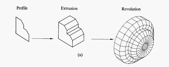
Boundary-representation (B-Rep)

In the B-rep method, first, a shape or a profile is defined. Second, a solid of revolution is generated about a given axis, or the profile is extruded in the given direction as illustrated below.

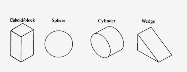
Constructive solid geometry (CSG)

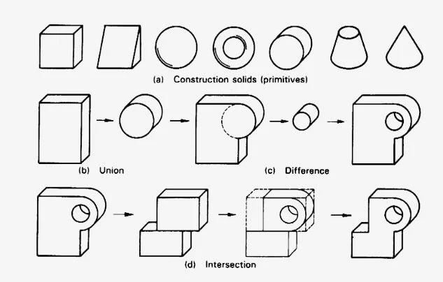
In constructive solid geometry (CSG), the modelers are equipped to provide a range of solid primitives which include cylinders, spheres, cuboids, wedges, and others. They can be defined at any size, position, and orientation as shown below.

Solid modeling systems such as I-DEAS and CATIA are not CSG modelers, though they are equipped with functions that are used for the generation of and operations on the solid primitives.

Likewise, other geometry construction facilities can be used to create profiles and thereupon generate models by extrusion or revolution of those profiles, thereby producing solids that may be referred to as primitives so that they can be modified by other generated solids and primitives using Boolean operations (figure a). Three such operations are as under.

• In the process of union, two construction solids are added and fused (Figure B)
• In the process of difference, one construction solid completely subtracts the other (Figure C).
• In the process of intersection, the two construction solids interact in such a way that the required solid contains volumes that are only overlapping, common, or intersecting. In contrast, the extraneous volumes are fully removed (Figure D).

Frequently Asked Questions